RINEX Reader
This was my first major project with python, most of this post will be taken from the assignment submission. The project was part of my GPS course in Undergrad, the project involved creating a python program to get an epoch by epoch least squares position solution of a GPS receiver using it’s observation and navigation RINEX files. This project was done with in part with Patrick Lasagne.
Objectives
- Develop python functions to process RINEX observations and navigation files and store the data in data structures.
- Develop python function to determine satellite position using the navigation files.
- Develop python functions to compute and apply ionospheric and tropospheric corrections, as well as satellite offsets, and apply them to observation pseudoranges where applicable.
- Run an epoch by epoch least squares adjustment to determine the location and clock offset of the receiver.
- Compute various DOP values using the covariance matrix from the least squares adjustment.
- Determine the accuracy and precision of the solution.
- Explain why the values were acquired.
Software Structure
RINEX stands for Receiver Independent Exchange Format, it is stored in an ascii format and contains GNSS Observations. The two RINEX files that the software reads are the observation and navigation files.
It was decided that the information stored in the observation and navigation files would be stored in a python dictionary data structure. A dictionary holds a set of unique “key-value” pairs that allow information to be accessed rapidly, without having to deal with messy array indices. The implementation is not important, all that must be kept in mind is that dictionaries allow the information present in the two RINEX files to be stored and later rapidly accessed with meaningful keywords at a later date. The only downside of dictionaries is that there is no reliable way to iterate through a dictionary in a certain order, to counteract this, each dictionary that may need to be iterated over also includes a list of keys corresponding to the key ‘LIST’ in the order they were placed into the dictionary.
The parsing of the RINEX navigation file is done line by line and character by character. Each element in the RINEX file is given a certain amount of spacing to fill up. This information on the spacing is found in the GAGE GROUP’s gLab RINEX file format description
Observation File Reader
The observation RINEX file contains all of the GPS receiver’s observations that it has collected over it’s setup time. The file is split into two components, the header, which contains important information about the receiver itself, and the data section, which contains phase and pseudorange observations to various satellites at various epochs.
Header Section
The header section contains information relating to the receiver, such as it’s position in a given coordinate system, it’s antenna height, or it’s make and model. It also contains clerical information pertaining to the observation set, and may include extra information present in comments. Most importantly, the header details the type of observations present in the RINEX file.
The header contains information for the first 60 characters (there are 80 on a line), the remaining 20 constitute a label which explains what is detailed in the previous 60 characters, each line is then terminated with a new line break (\n). To fully parse the header, the RINEX file is read in line by line. At each line, the label is checked to see what kind of header information is present on that line, this continues until END OF HEADER was reached, at that point, the software would switch from trying to read the header, to trying to read the observations. While the software attempts to read the header, it consults the last word of the label, and attempts to match it with a predefined list present in the software (with HTYPER method). In the event that two or more label types have the same last word, then the second last word is used instead. Once the label is identified, the software parses the line according to it (with ASSIGNDIC). The values present are extracted from the line with direct indexing (ex, character 0-16), are assigned meaningful “keys”, and are placed in the dictionary. In th event that a key already exists (or a multi-line label is reached), the value at the key is changed depending on label type. For example, if a COMMENT label is reached, the current string value stored at the key ‘COMMENT’ has the new value appended to it’s end. In the event # / TYPES OF OBSERV occurs on more than two lines (with more than nine observation types), the list that holds the observation types has the extra values appended to it. While all information in the header section was stored in the obsHead dictionary, only a few important keys present in the header are used in the software, they are:
| Key | Value | Description |
|---|---|---|
| ‘POS’ | Dictionary with sub keys ‘X’, ‘Y’, and ‘Z’ | Contains the X, Y, and Z position of the receiver. |
| ‘OBSTYP’ | Dictionary with sub keys ‘NUM’ and ‘OBS’ | ‘NUM’ contains the integer number of satellites ‘OBS’ contains a list of the two alphanumeric GPS observation types (ie ‘C1’, ‘P1’) |
Data section
The data section contains the epoch by epoch observations by the receiver to the satellite. It contains measurements for several satellites, the measurements included are limited by what is present in the ‘OBS’ observation list mentioned above. The reader reads the first line, which has the epoch, the total number of satellites and the list of the satellites. The epoch is made into a key in the form ‘YY:MM:DD:HH:MM:S.sssssss’, it maps to a dictionary that will be used to include all satellite observations. The reader then uses the number of satellites present and the number of observations expected to determine how many lines remain in the observation block. It then creates a list of the satellites andd uses each three-digit PRN value as a key in the dictionary paired with the epoch key mentioned above. The reader reads line by line and creates a dictionary that is matched to the correct PRN key for each satellite PRN. The dictionaries referred to by the PRN keys are then filled with key value pairs that refer to the observation information stored in the observation block. While all the information was stored in the observation dictionary only some of it was used, the key descriptions and the dictionary structure can be seen below.
| Key | Value | Description |
|---|---|---|
| ‘YY:MM:DD:HH:MM:S.sssssss | Dictionary with sub keys ‘PRN’,‘PRN’,‘PRN’, and ‘LIST’, ‘NUMSAT’ | The key refers to the observation block epoch. It maps to a dictionary which contains dictionaries referred to by satellite PRN numbers, each dictionary corresponds to a different satellite in the observation block. ‘LIST’ maps to a list of all satellite PRN numbers (for iterating) ‘NUMSAT’ refers to the integer number of satellites. |
| ‘PRN’ | Dictionary with sub keys ‘C1’, ‘P1’, ‘P2’, etc | Contains the observations for the given satellite at the given epoch. |
Dictionary Structure
{
    '07:1:1:0:0:0.0000000':{
        'G06':{
            'C1':20857582.237,
            'P1':20857582.016,
            'P2':20857580.516,
            },
        'G07':{
            'C1':20418227.176,
            'P1':20418226.502,
            'P2':20418225.415
            },
        'G10':{
            'C1':23445664.779,
            'P1':23445663.158,
            'P2':23445663.052,
        },
        'LIST':['G06','G10','G07'],
        'NUMSAT':10
    },
    '07:1:1:0:0:30.0000000':{
        'G06':{
            'C1':20868360.224
            ...
        }
    }
}
Navigation File Reader
Header Section
The header file contains metadata information about the RINEX file such as the RINEX version. The line identifier in header has reserved space of 20 characters at the end of the line. Each RINEX file has 80 characters per line therefore the location of the header labels are always known. For each header label the location of the variables is defined by the index of the character spacing. For each label a dictionary key is defined as the variable value corresponding to the label is stored. Besides the RINEX version the header contains comments about the RINEX file, and 3 optional information such as the emphemeris coefficients of the Ionosphere alpha and beta. Also optionally included in the header is the clock offset coefficients of UTC from GPS and the number of leap seconds the current GPS time is from UTC. The end of the header is defined by the label ‘END OF HEADER’ once this is reached then parsing of the navigation data begins.
Data Section
The navigation data is sorted in the RINEX file by the GPS PRN number then epoch the ephemeris data is valid for. Again the spacing for each element of the broadcast is defined for every line. The label for the PRN key is defined for the first 2 space of the line after the header. Once the PRN number is parsed then the lines are counted from that point on. Each element of the line has certain index and spacing, then the data is parsed until the 8th line is reached and a new PRN number is parsed. Each broadcast contains 29 variables that the satellite broadcasts. These 29 variables are given in a block of 8 lines and 4 columns, one of the spaces is for the PRN number and the epoch while the other 2 spaces of the 32 spaces are left empty in the RINEX 2.11 version.
The data is collectively stored with a nested dictionary, where the top most key is the GPS PRN number, then the data blocks are divided by subkeys of the epoch that the broadcast data is valid for.
| Key | Value | Description |
|---|---|---|
| ‘PRN’ | Dictionary with sub keys epoch | Contains the 29 navigation parameters and broadcasted navigation information by the satellite. |
Navigation Dictionary Structure
{
    'GO1':{'10:1:1:16:0:0.0':{
        'Cic':5.587935447693e-09,
        'Cis':7.636845111847e-08,
        'Crc':183.21875,
        'Crs':-165.46875,
        'Cuc':-8.651986718178e-06,
        'Cus':1.038610935211e-05,
        'Deln':5.447369761959e-09,
        'Ecc':0.003840734250844,
        'Fit_int':4.0,
        'GPS_W':1564.0,
        'IDOT':-7.000291590243e-11,
        'IODC':51.0,
        'IODE':51.0,
        'Io':0.9635689853388,
        'L2_CC':1.0,
        'L2_P':0.0,
        'Mo':0.0841761497488,
        'OMEGA':-0.1005044703918,
        'OMEGA_DOT':-7.951402636407e-09,
        'Omega':0.9428572252394,
        'SV_Acc':2.0,
        'SV_CLB':-7.538078352809e-05,
        'SV_CLD':-3.069544618484e-12,
        'SV_CLR':0.0,
        'SV_Health':63.0,
        'SqrtA':5153.668302536,
        'TGD':-1.909211277962e-08,
        'TOE':489600.0,
        'Trans_time':487788.0
    }}
}
Satellite Position
To compute the receiver coordinates, first the coordinates of the satellite must be determined. It is a fairly straightforward process of determining the satellite coordinates, the Keplerian elements of the satellite is broadcasted in the Navigation file. Each satellite in the GPS constellation does this broadcast of all the GPS satellites in the constellation and broadcasts its position prediction in orbit for each two hours. Once all the 29 parameters in the RINEX navigation file are read the process of determining the satellite position occurs in the module satpos.py
The process of determining the satellite positions are outlined in detail in ICD document. The algorithm is defined in section 20.3.3.4.3 User Algorithm for Emphemeris Determination Pages 103-105. The equations are defined in Table 20-IV of the ICD document.
The SatPos function strictly follows the defined guidelines, except a few tweaks for the time variable used in the process of determining the satellite position is in GPS seconds of the week, which is the number of seconds that have passed since the start of a GPS week which is on Saturday midnight. The eccentric anomaly defined in the algorithm is solved using an iterative process, the Eccentric anomaly is calculated until the difference of the current value and the previous value are smaller than a defined threshold which in the software was defined to be 0.000000000001. Once this condition is satisfied the current Eccentric anomaly is saved and used for further calculations.
Once all of the Orbital parameters are determined and the position of the satellite in the orbit determined the final output of the function is the ECEF coordinates of the satellite in interest.
Corrections
Ionospheric Correction
The effect due to the ionosphere can be mitigated in two ways. If using a single frequency receiver, the delay caused by the ionosphere can be modelled with the Klobuchar model. Since the software does not attempt to adjust a single frequency receiver observations, the Klobuchar model will not be explained here. When using a dual frequency receiver, the delay due to the ionosphere can be nearly mitigated with a linear combination of the two equations, one on each frequency. The equation for the Ionofree linear combination that removes most of the ionospheric effect is:
$$ [PR=\frac{PR_2-\gamma PR_1}{1-\gamma}] $$
PR is the iono free corrected pseudorange, PR_1 and PR_2 are the pseudorange observations on two frequencies, and gamma is the squared ration between the two carrier wave frequencies given by:
$$ [\gamma =(\frac{f_1}{f_2})^2 = (\frac{1575.42}{1227.6})^2 = (\frac{77}{60})^2 ] $$
Tropospheric correction
When the GPS signal travels through the atmosphere it is refracted by the medium, which in turn delays the signal, this refraction is mostly caused by the moisture content in the Troposphere. This delay can be modeled and determined so it can be used to correct the pseudorange observations. The model used in the software was the Saastamoinen Closed Form model. The model is defined as:
$$ [dtrop=\frac{0.002277}{cos(z)}[P_0 + (\frac{1255}{T} + 0.05)e_0 - tan(z)^2]] $$
Where dtrop is the tropospheric correction to the pseudorange in meters, z is the zenith angle from the receiver to the satellite of interest, P_0 is the atmospheric pressure in mbar, T is the temperature in Celsius, and e_0 is the water vapour pressure in mbar.
This element of the software did not function properly, it was causing significant deviations in the order of thousands of meters in some cases in the solution therefore the tropospheric delay was omitted in the final solution.
Least Squares Filter
The receiver coordinates and it’s clock offset must be estimated using a epoch by epoch Least Squares solution. This will allow for a iterative solution from an over determined system, that is, an equation system where there are more equations that unknowns (and thus, more than one correct answer). Least Squares ensures that the solution will be the one that fits the model best.
The mdoel equation is the formula for a psuedo range, shown below that describes the geometric explanation of a pseudo range. It includes a geometric component inside the square-root term, as well as a time component.
$$ [PR=\sqrt{(X_s - X_r)^2 + (Y_s - Y_r)^2 + (Z_s - Z_r)^2} + c(t_r - t_s)] $$
PR is the pseudorange between the satellite and the receiver, it can be likened to the geometric range, plus a correction in the time domain. The square root term is the geometric range from satellite to receiver, where terms with a subscript “s” are satellite coordinates, and the terms with a subscript “r” are the receiver coordinates. The coordinates are assumed to be in the same coordinate system. The three receiver coordinates are part of what the least square adjustment attempted to estimate. c is the speed of light in meters per second and was provided in the ICD. The variable t_r is the time offset on the receiver, and is another parameter that must be solved for, finally t_s is the satellite vehicle offset, and provides a small error that must be compensated for.
Once the model has been chosen, it must be parameterized, that is observables, unknowns, and constants must be chosen.
The observables were chosen to be the pseudoranges (PR), they form a vector of observables l seen below
$$ l = [PR_1, PR_2, PR_3 … PR_n] $$
The receiver position in the x, y, and z, as well as it’s clock offset were chosen to be the unknowns.
$$ x = [X_r, Y_r, Z_r, t_r] $$
The constants were chosen to be satellite positions, and the satellite clock offset. Once the observables and unknowns were chosen, a suitable least squares model had to be chosen. Since all observables are present on one side of the equation, and the other side of the equation is a function of only unknowns and constants, parametric adjustment was chosen with the model.
$$ l = f(x, c) $$
Because the pseduorange equation is a non-linear equation (Variables are raised to a power other than 1 or -1), the equation must be expanded using Taylor Series Expansion using only the first two terms.
$$ f(x) \approx f(x0) + \frac{1}{1!}\left. \frac{df}{dx}\right|_{x=x_0} ( x - x_0) $$
Which consists of an initial estimate f(x0) of the unknown parameter x, with a correction scaled by the difference between the difference of the “true” value x and the initial estimate. The initial estimates were chosen to be the listed X, Y, and Z position of the station in the header, with a time offset of 0. In least squares adjustment, the difference between the “true” value and the estimated one is given by delta. The correction to teh estimates is what is solved for in each iteration. Iterations usually continue until delta is significantly small, but in the case of this particular adjustment, delta is only iterated a few times. The linearized model also contains a part about the partial derivative of the function with respect to a variable x, in least squares adjustment, x is a vector, and a matrix must be composed of the partial derivatives of the functions with respect to each unknown in a vector. This matrix is called the first design matrix (A), and can be seen below.
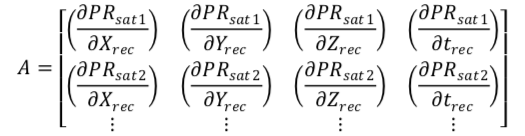
Where PR_sat1 is the pseudorange function of the first satellite, PR_sat2 is the pseudorange function of the second satellite, and so on. X_rec, Y_rec, Z_rec and t_rec are the unknowns mentioned earlier.
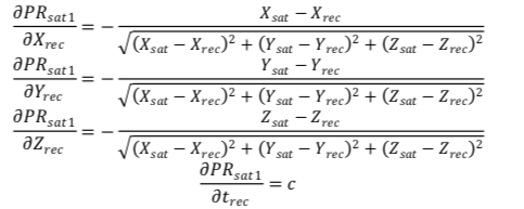
The partial derivatives of the pseudorange equation with respect to the each unknown can be seen below:
One other matrix must be created before delta can be solved for, the misclosure vector w which is the measure of how well the unknown estimations fit with the model and the pseudorange observations, w is given by:
$$ w = l - f(x_0) $$
Where l is the matrix of observables, and f(x_0) is the matrix of pseudoranges computed using the pseudorange model equation, with the estimated receiver coordinates and clock offsets. Once the required matrices have been created, delta can be given by:
$$ \delta = (A^TA)^{-1}A^Tw $$
Everytime delta is calculated, the initial estimations must be updated, delta is added to x_0, w and A are recomputed and the iteration continues.
After a solution for an epoch has been found, the covariance matrix of the unknowns (C_x) can be computed as :
$$ C_x = (A^TA)^{-1} $$
It is a 4x4 matrix which contains the covariances of each unknown to the themselves and all other unknowns, shown below:
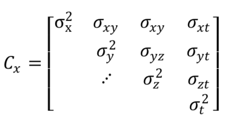
It can be seen that the variances of the unknowns are present in the diagonal components, and that all off diagonal components are the covariance’s between unknowns. The diagonal variances will be used to compute the DOPs of the epoch, which will be explained in the next section.
The adjustment process is completed for each epoch. Initial estimations from the previous epoch are used as estimations for the next epoch.
Analysis Terms
Standard Deviation
The standard deviation is a statistical measure of accuracy of a given variable. It defines a confidence interval of where the true value of the variable can lie within. One standard deviation defines 68% confidence interval where the true value of the variable lies within. For the position solution each of the coordinates are defined with the value and it’s standard deviation. The standard deviation is a product from the Least Squares process of the position solution. It is the square root of the diagonal elements of the Covariance matrix of the unknowns, which in this case are the X, Y, and Z and the clock offset.
Dilution of Precision
The Dilution of Precision is a measure of precision of the solution. It is defined simply as the trace of the covariance matrix of the solution. The two types of DOPs used in this report are Geometric DOP (GDOP) and Position DOP (PDOP). The DOPs are defined as:
$$ GDOP = \sqrt{\sigma_x^2 + \sigma_y^2 + \sigma_z^2 + \sigma_t^2c^2} $$
$$ PDOP = \sqrt{\sigma_x^2 + \sigma_y^2 + \sigma_z^2} $$
Analysis
This section describes the analysis of the solution for the data used for a test site.
Test Site ALBH
The RINEX dataset were provided by the Teaching Assistant, the station used for the positioning solution was designated ALBH. The station is location near Victoria, British Columbia. ALBH is a continuously tracking GNSS site, it is part of the Western Canada Deformation Array (WCDA) it is also part of the Canadian Active Control System(CACS). The published coordinates of the site is given in the Natural Resources Canada’s CACS website. The ECEF coordinates are published as:
X = -2341333.003 +- 0.0007
Y = -3539049.514 +- 0.0008
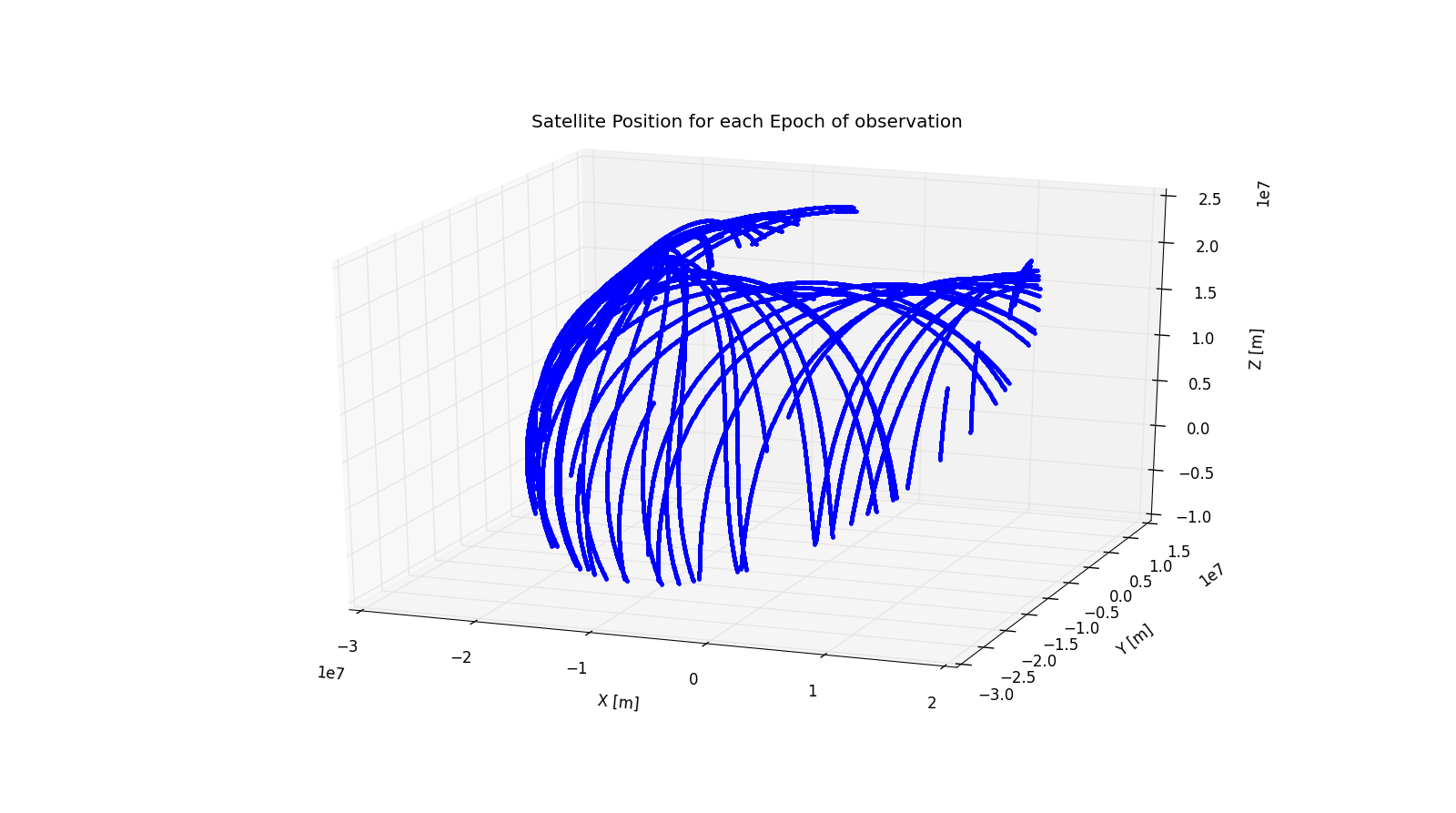
Z = 4745791.300 +- 0.0009Satellite Positions
As described before the satellite positions for every epoch of the recorded observations have to be calculated. The RINEX observations are recorded for every 30 seconds, therefore there are quite a number of satellite positions to be determined about 2600 epochs of measurements. A good way of ensuring the satellite positions are being calculated correctly is to visualize the satellite positions. The expectation of these plots is to follow a similar path of the sun rise and fall motion.
Positions
The final solution of the receiver coordinates can be plotted to visualize the quality of the solution. The pyplot library was used for all graphical plotting and image generation. Below is a scatter 2D plot of the receiver X and Y coordinates.
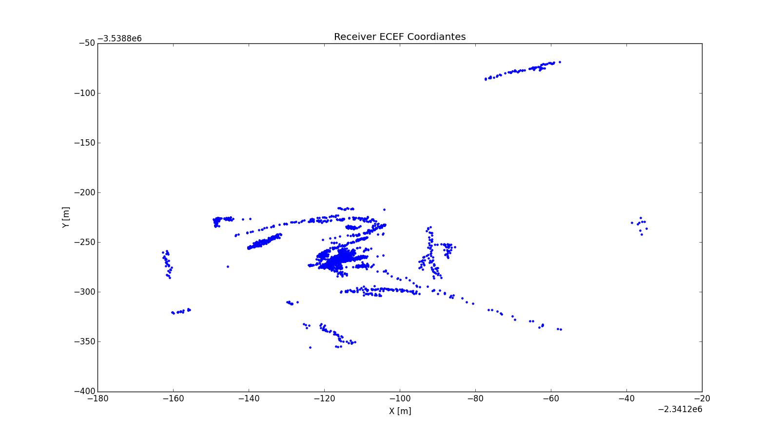
Looking at the above figure there seems to be an irregularity with the position solutions. The expectation of the final solutions would be a general agreement of the position therefore the scatter plot should show a cluster of positions centered around a region. Looking at Figure 2 that is not the case, there are several position several hundreds of meters away from the centered cluster of points around the published coordinates. The expected accuracy of the Standard Position Solution are meter level the final solutions outputted do not seems to satisfy the quality. Further investigation has to be made to understand this anomaly, there could be various factors resulting this deviation. It should be kept in mind that the tropospheric delay was not corrected for these solutions because of divergence in the final solution with the tropospheric delay turned on position solutions were different in the range of kilometers. One interesting characteristic from the plot that can be noticed is there are streaks in the positions. This hints towards a correlation between time, therefore there has to be a blunder in the programming where it is obtaining an incorrect satellite position or an incorrect time. Due to time constraints the debugging of the code was not completed.
Another piece of evidence that can be used to visualize the discrepancy in the solutions is the coordinate difference from the published coordinates of the solution.
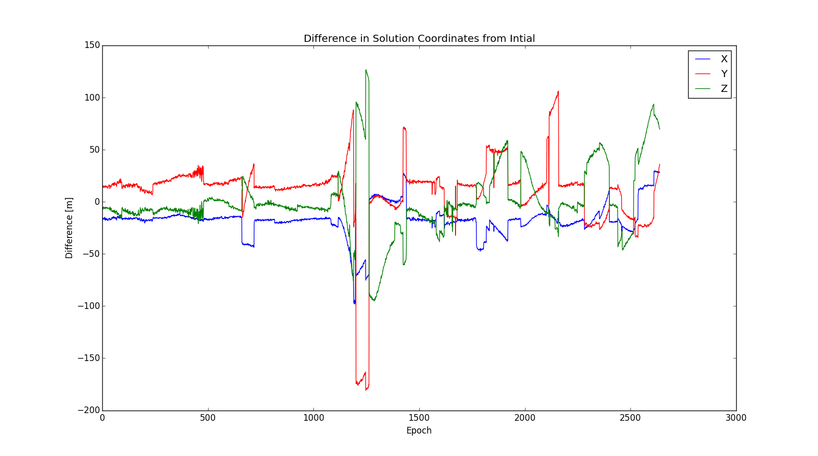
As one can notice from the above figure the initial solutions seem to have a stable deviation of about meter level for X and Z, 10s of meters for the Y component for about the first 1000 epochs then the coordinates deviate to 100 of meters past the 1100th epoch. This anomaly hints to the general time to which is causing the discrepancy in the position solutions.
The solutions were averaged to obtain a general estimate of the position of ALBH, below are the tabulated results.
| Component | Value | Standard Deviation |
|---|---|---|
| X[m] | -2341315.307 | 15.103 |
| Y[m] | -3539059.522 | 34.744 |
| Z[m] | 4745791.669 | 31.694 |
| t[s] | -3.39126190338e-08 | 3.06918042012e-07 |
To get a general sense of how different the solutions are from the published ones the difference between the solutions were determined and tabulated below.
| Component | Coordinate difference[m] |
|---|---|
| X | 17.695 |
| Y | -10.008 |
| Z | 0.369 |
DOP Values
The DOP of the final solution can be visualized to see if there is any correlation between the epoch when the discrepancy began. The figure below illustrates the GDOP values for each epoch of the solution.
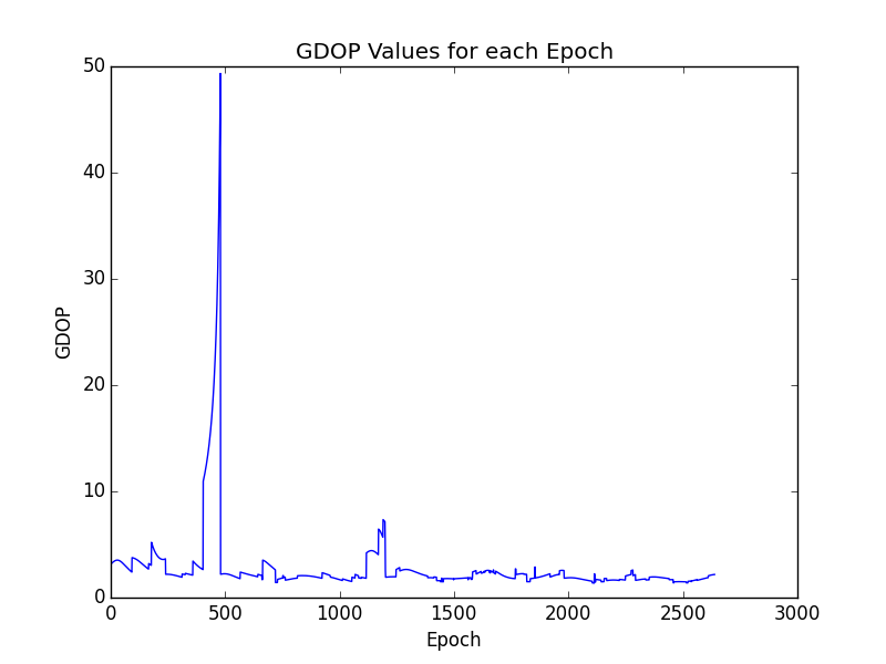
Looking at the above figure there is quite a noticeable discrepancy in the GDOP of the solution for a period of time around the 500th epoch. This spike in the GDOP value although does not correlate with teh discrepancy illustrated in the figure with the coordinate difference. For the rest of the solution the GDOP seems to have a reasonably low and workable value. The average GDOP for the timeline of the observation file was 2.76. Which is quite good but looking at the GDOP plots it still doesn’t provide insight on the deviation of the final coordinates.
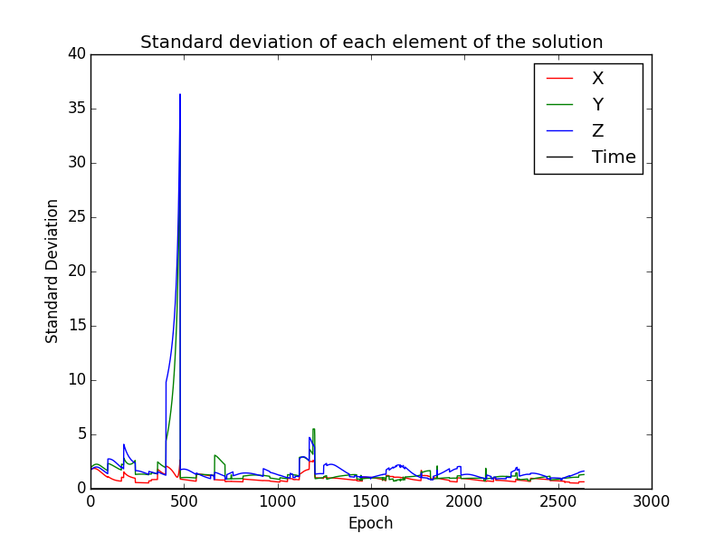
Figure above illustrates the standard deviation of each of teh elements in the solution. It can be clearly seen the huge spike in the GDOP plot are mostly contributed by the Y and Z component of the solution. This narrows down the component to which is causing the deviation of the position of the receiver with the published one. As mentioned before due to time constraints the problem could not be pinpointed and solved.
Conclusion
This report involves all the software components needed to compute a Standard Positioning Service GPS navigation solution. The software was tested for a test case of observation data, although a position was outputted, the quality of the solution was not acceptable. The software bugs that caused the deviation could not be determined over the timeline of this project due to time constraints. If there was more time the tropospheric delay of the GPS signal could be implemented as well as tested as well as the Klobuchar model for determining the ionospheric delay for a single frequency receiver.